Transect estimates

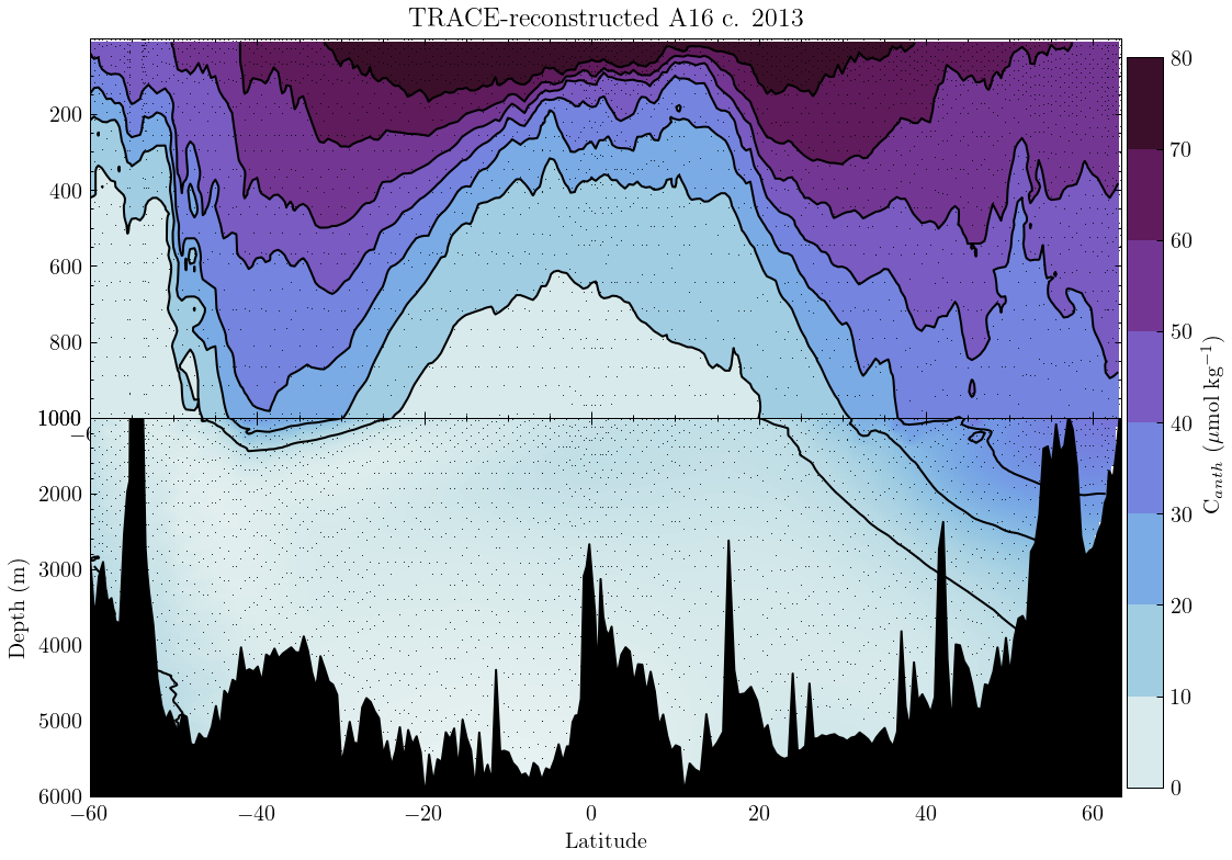
Estimates of age and C_anth may be obtained from an entire transect, as demonstrated here for the GO-SHIP A16 transect, using data from the 2013-2015 reoccupation. Users wishing to replicate this analysis should obtain the NETCDF bottle files from CCHDO, or (by modifying the data preparation as in this script) using *_hy1.csv files as demonstrated in the neutral_density package.

Input and preparation

Start by importing necessary dependencies. You may need to install some of these in addition to trace.

import pandas as pd
import numpy as np
import xarray as xr
from tracepy import trace
from seawater import dpth # deprecated by TEOS-10, should use GSW

Import datasets containing A16 botle data, then rearrange into a clean Pandas dataframe. We're selecting for QC flag 2, indicating "good" data.

a16n = xr.open_dataset("path/to/33RO20130803_bottle.nc")
a16s = xr.open_dataset("path/to/33RO20131223_bottle.nc")
combined_length = len(a16n.N_PROF) * len(a16n.N_LEVELS) + len(a16s.N_PROF) * len(
    a16s.N_LEVELS
)
latlist = np.concatenate(
    [
        (
            np.ones((len(a16n.N_PROF), len(a16n.N_LEVELS)))
            * a16n.latitude.data[:, None]
        ).ravel(),
        (
            np.ones((len(a16s.N_PROF), len(a16s.N_LEVELS)))
            * a16s.latitude.data[:, None]
        ).ravel(),
    ]
)
lonlist = np.concatenate(
    [
        (
            np.ones((len(a16n.N_PROF), len(a16n.N_LEVELS)))
            * a16n.longitude.data[:, None]
        ).ravel(),
        (
            np.ones((len(a16s.N_PROF), len(a16s.N_LEVELS)))
            * a16s.longitude.data[:, None]
        ).ravel(),
    ]
)
input_df = pd.DataFrame(
    {
        "lat": latlist,
        "lon": lonlist,
        "pressure": np.concatenate(
            [a16n.pressure.data.ravel(), a16s.pressure.data.ravel()]
        ),
        "year": np.ones((combined_length)) * 2013,
        "sal": np.concatenate(
            [
                a16n.bottle_salinity.where(a16n.bottle_salinity_qc == 2).data.ravel(),
                a16s.bottle_salinity.where(a16s.bottle_salinity_qc == 2).data.ravel(),
            ]
        ),
        "temp": np.concatenate(
            [
                a16n.ctd_temperature.data.ravel(),
                a16s.ctd_temperature.data.ravel(),
            ]
        ),
    }
)
# input_df = input_df.dropna(how="any")
input_df["depth"] = dpth(input_df.pressure, input_df.lat)  # pressure to depth

C_anth Estimation

Now that the transect has been rearranged into "long" format (i.e. a number of columns of data), these columns can be readily accessed in the required order and converted to the necessary numpy arrays. Inputting the coordinates, salinity, temperature, and times of measurement into trace, yielding a CF-compliant xarray dataset containing C_anth estimates, along with age and associated metadata.

output = trace(
    output_coordinates=input_df[["lon", "lat", "depth"]].to_numpy(),
    dates=input_df.year.to_numpy(),
    predictor_measurements=input_df[["sal", "temp"]].to_numpy(),
    predictor_types=np.array([1, 2]),
    atm_co2_trajectory=5,
    verbose_tf=True,
)

These estimates can be plotted with your section plotting tool of choice, resulting figures resembling this example (derived from the TRACE demos scripts):